Black-hole weather: forecasting accretion flows with a trust horizon

pinneapple_physics.blackhole reproduces and extends Duarte, Nemmen & Navarro (2022), Black hole weather forecasting with deep learning: a pilot study (MNRAS 512, 5848; arXiv:2102.06242; code, MIT: black-hole-group/DL_BH_fluids). The original work trained a U-Net on hydrodynamic simulations of the hot, radiatively inefficient gas around a black hole and forecast the flow about 10⁴ times faster than the fluid solver. This module adds what the weather work in PINNeAPPle asks of any forecast: for how long can it be trusted, and can we tell without the truth? Issue #399.

Pieces

module	what it does
hydro	AccretionFlow: axisymmetric viscous hydrodynamics around a Schwarzschild black hole (Paczyński-Wiita potential, α-viscosity "SS" or "ST", equilibrium torus), finite volume (HLL, MUSCL, SSP-RK2) on a log-r grid; bondi_pw: exact transonic Bondi accretion for validation
forecast	DuarteUNet (layer-for-layer port of the original), DensityCodec, make_blocks, train_forecaster, rollout, lead_time_scores, trust_horizon, MassEnvelope
twin	accretion_scene: the flow revolved in 3D as a cutaway for PINNeAPPle-Twin3D, simulation and forecast side by side, trust signals as sensors
capture	capture_twin: records the Twin3D viewer (headless Chromium) to frames for GIFs

The simulations

The paper's training data are PLUTO runs (Almeida & Nemmen 2020) that are not reachable from every environment, so examples/black_hole_weather/simulate.py regenerates the same kind of flow with the library's own solver:

• units G = M = c = 1; potential Φ = −1/(r − 2), which places the innermost stable orbit at r = 6;
• adiabatic gas (γ = 5/3) without cooling, total energy evolved so viscous heat stays in the gas;
• viscosity only in the azimuthal stresses T_rφ, T_θφ (Stone, Pringle & Begelman 1999), with ν = α c_s²/Ω_K ("SS") or ν = α r^1/2 ("ST");
• initial equilibrium torus with l(R) = l_c(R/R_c)^a (pressure maximum at R_c = 20, inner edge 12) in a cold atmosphere; r from 4 to 400 GM/c², 128 × 64 cells;
• runs named like the paper's, PL{a}{SS|ST}{α}.

Validation (tests/test_blackhole_weather.py):

• mass and angular momentum close to round-off (10⁻¹⁶) once the boundary fluxes are counted;
• a uniform pressure at rest stays at rest (exact geometric source terms);
• the inviscid torus holds its equilibrium;
• exact Bondi accretion in the Paczyński-Wiita potential stays steady: accretion rate within 0.5 % and density within 0.2 % (median) over 2000 GM/c³.

As in other black-hole codes, the tenuous atmosphere has floors and a speed / temperature ceiling (v_max, t_cap); AccretionFlow.capped counts the cells where they act (≈1 % of the cells, next to the hole).

The forecaster

Five consecutive density snapshots go in as channels, the next five come out; the density is log-normalised and the outer atmosphere and polar cells are cropped, as in the original. The loss is MAE + α·MAE(pixels with y > 0.5) (the paper's multi-simulation loss; its one-simulation loss uses pixel boxes of its own grid, which do not transfer).

Trust

• Trust horizon. Iterative rollouts from many start times; per lead time, the error of the forecast against persistence and against the time-mean flow, and the anomaly correlation (ACC) with the simulation. The horizon is where the ACC drops below 0.6 (the weather convention).
• Mass check, no truth needed. The gas in the forecast window can only change by what crosses its edges, and the training simulations show how fast that ever happens (MassEnvelope). A rollout whose mass moves faster is creating or destroying gas — the "artificial mass injection" the original authors identify as the cause of drift — and the first lead where that happens is a trust limit available in operation.

3D digital twin

from pinneapple_physics.blackhole.twin import accretion_scene
sc = accretion_scene(grid, {"simulation": logrho_true, "forecast": logrho_pred}, times, r_view=60,
                     sensors=[{"id": "forecast error", "panel": "forecast", "series": err, "envelope": (0, err_max)}])
sc.export("out/bh_twin")            # pinneapple_twin3d.serve("out/bh_twin") -> browser

The axisymmetric flow is revolved into a 3/4 cutaway (two meridional planes and the equatorial sector) around a black sphere at the event horizon. The viewer accepts ?field=log10_density&cmap=inferno&view=1,0.75,-1&range=-6,0 to open on that view.

Interstellar view (general-relativistic ray tracing)

raytrace.Camera.trace integrates the null geodesics of the Schwarzschild metric once per camera: each ray stays in a plane through the hole, and u = 1/r obeys u'' = 3u² − u, solved by RK4 with arc-length-limited steps. raytrace.render then integrates the emission of any (r, θ) density / temperature / velocity frame along those rays. It includes:

• the gravitational and Doppler redshift (I ∝ g⁴);
• optional grey absorption;
• a colour temperature that follows g;
• a procedural star field that is lensed with the flow;
• a film-like bloom.

The tests check that the shadow edge sits at the critical impact parameter b = 3√3 M and that a thin disc shows its far side lensed above the shadow, as in Interstellar (James et al. 2015).

The twin also renders in Blender: Scene.render_blender / render_blender_frames (Cycles, pip install bpy).

Resolution study, zoo dataset and retrained forecaster

The reference was checked on four grids (90 × 45 to 256 × 128, ratio √2, three seeds each, the same seeded perturbation on every grid). The tools are in the library:

• convergence.resolution_study: conservative remap, Richardson order and GCI through pinneapple_analysis.verification, and statistical convergence;
• dataset: the zoo dataset blackhole_riaf_density_256, whole trajectories per split;
• forecast.train_on_trajectories: rollout loss, input noise, mass penalties, resumable;
• skill.evaluate_skill: persistence, climatology and DMD baselines, moving-block bootstrap intervals, physics checks;
• figures.

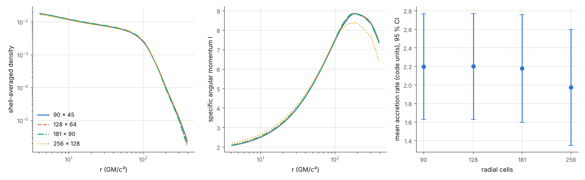
• The means converge within their 95 % bands: the accretion rate is 2.18 ± 0.58 on 181 × 90 and 1.97 ± 0.63 on 256 × 128, and the mass in the window and the density slope also agree.
• The profiles are not in the asymptotic range. From 181 to 256 they change by 4-11 %, against 0.5-2.5 % between the coarser grids, and l/l_K rises 3.8 % beyond its band. The likely cause is that the speed and temperature ceilings act on more cells as the resolution grows. These changes are the stated uncertainty band of the data.
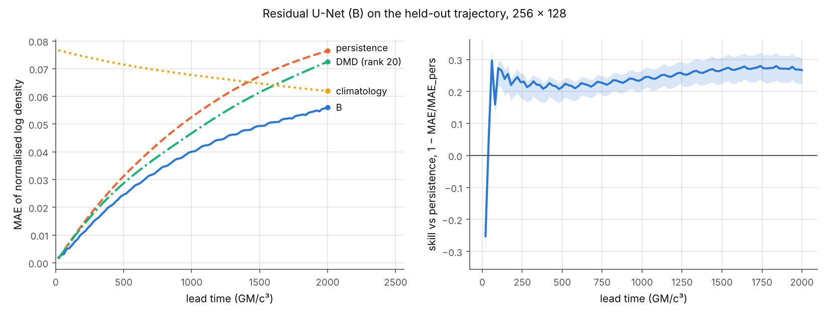
• The forecaster is not shipped. Retrained on 256 × 128 trajectories with replicate padding, a rollout loss and a mass penalty, it beats persistence with 95 % confidence from 60 to 2000 GM/c³ (skill 0.27 at 2000 M) and beats DMD. But it breaks the mass envelope of the training runs in 14-54 % of the frames.

Details and every number: examples/black_hole_weather/README.md, section "Zoo version".

Results of the first version

The port of the paper's U-Net does not beat persistence at the 20 GM/c³ frame spacing used here. It loses or gains 4-6 % of the gas per frame, which the mass check flags at the first frame. The residual variant (predicting the change) beats persistence over the whole 1200 GM/c³ test rollout: 45 % lower error in distribution and 21 % lower for an unseen α. Numbers, figures and GIFs are in examples/black_hole_weather/README.md.