3D studio and external flow

Two layers turn any geometry and its physics into pictures people understand: pp.viz, which renders, exports and browses, and pp.cfd, which runs OpenFOAM around any body. They came out of the Aircraft Design Optimizer (apps/aero_optimizer) and work the same way for a car, a building, a heat sink or a beam.

import pinneapple as pp

scene = pp.viz.Scene.from_file("result.frd")          # any result pinneapple_data.cae reads, or an STL/OBJ
scene.save("result.glb")                              # glTF with the fields; .usda for Omniverse; .stl
pp.viz.render(scene, "stress.jpg", field="STRESS")    # Blender Cycles, jet scale, colour bar
pp.viz.web_viewer(scene, "viewer/")                   # interactive page (python -m http.server -d viewer)

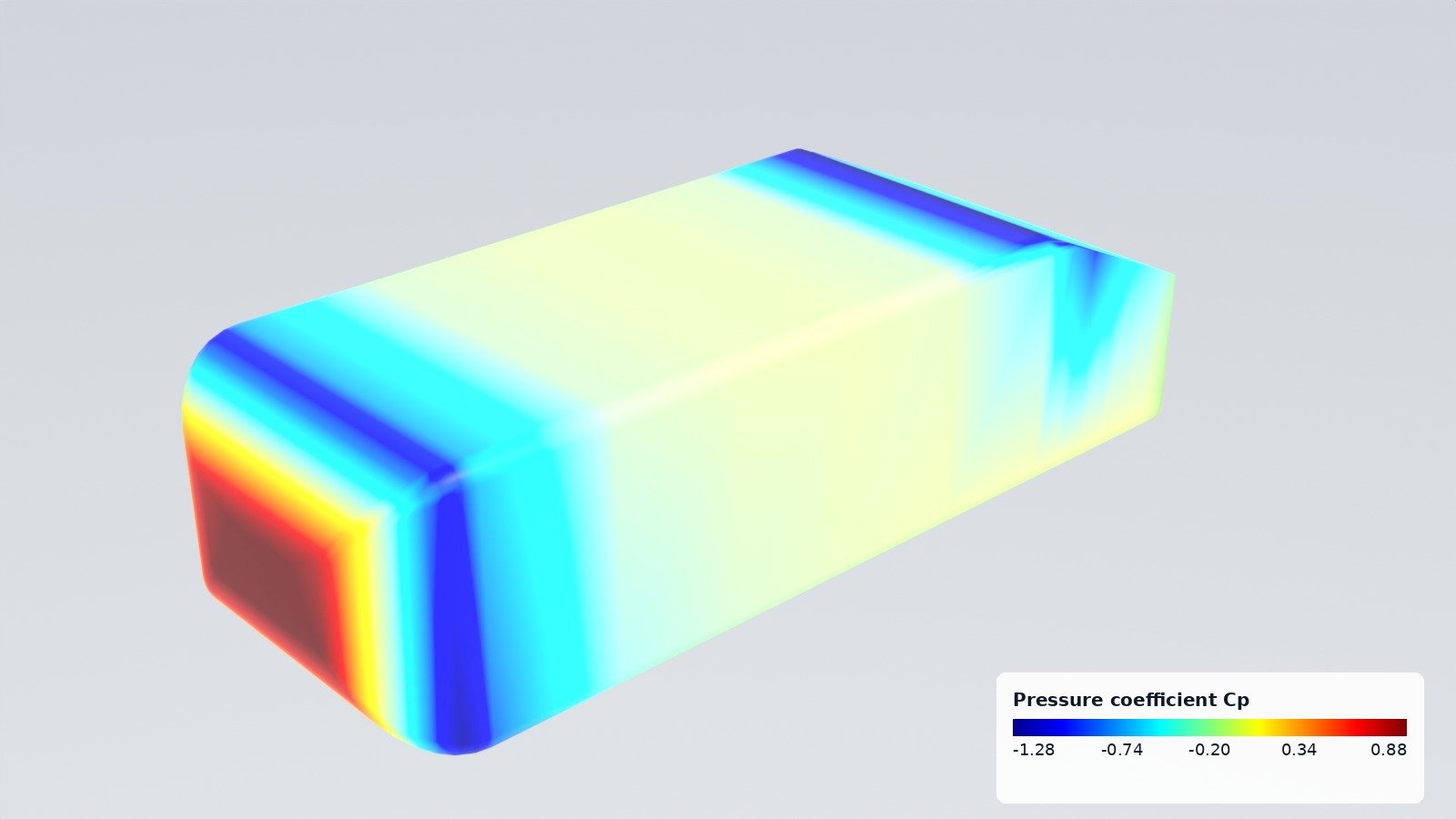
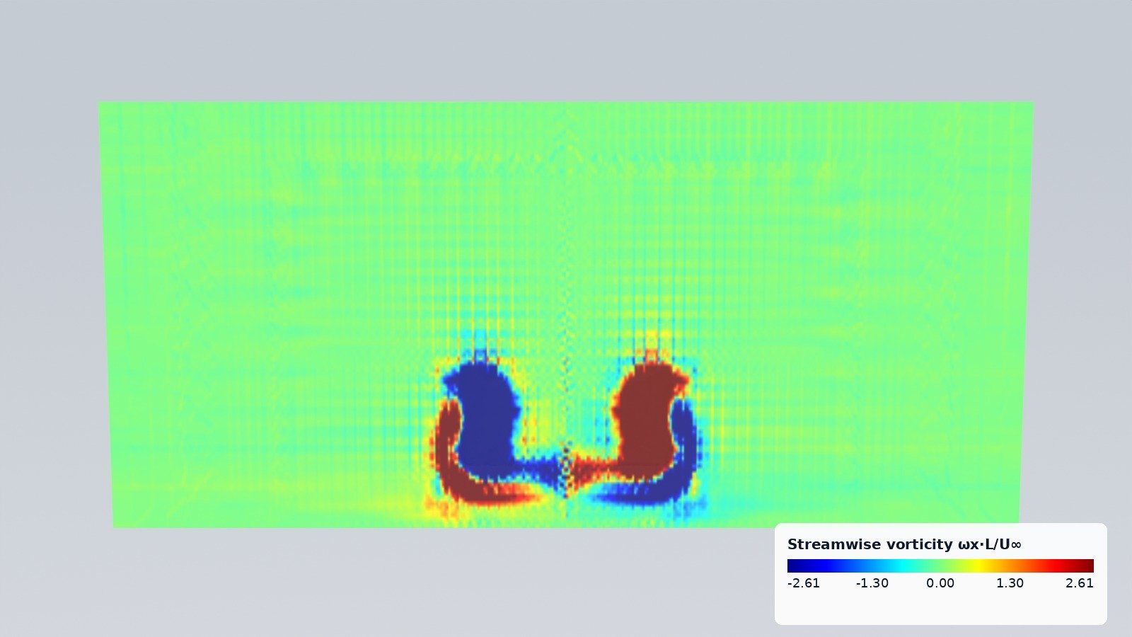
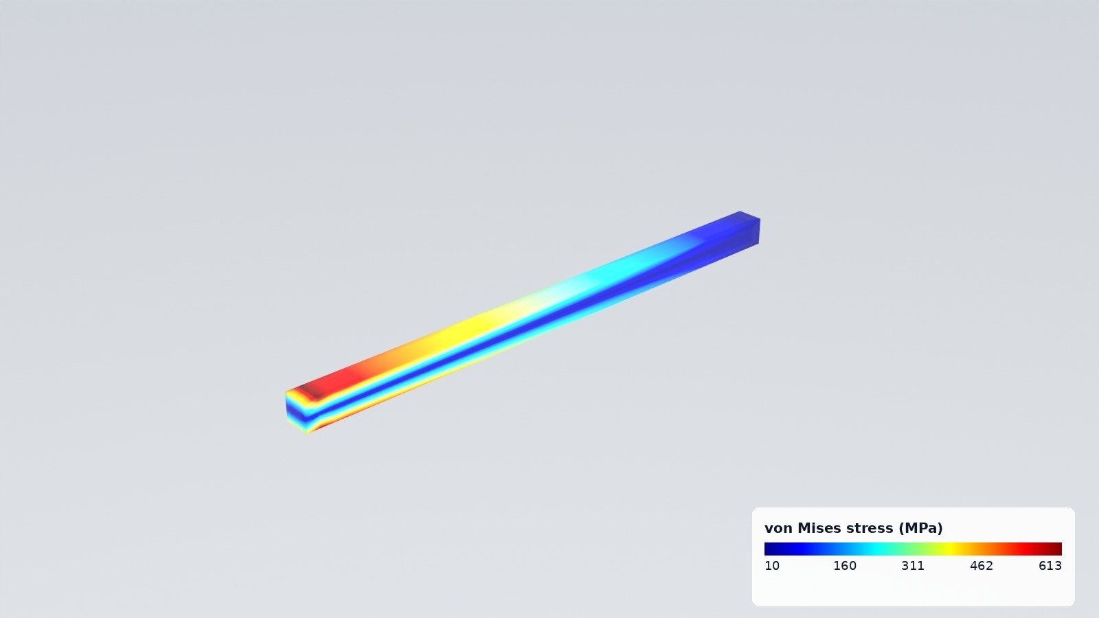
Scene

A Scene holds surfaces (vertices, triangles, a material and per-vertex fields), polylines with values (streamlines) and slice planes (a value grid on a rectangle, NaN where there is no fluid).

Build it from	Call
STL (binary/ASCII, one surface per solid), OBJ	Scene.from_file("part.stl")
glTF/GLB (node transforms applied; float attributes _NAME become fields)	Scene.from_file("model.glb"), axes="aircraft" for files written in aircraft axes
VTK PolyData .vtp (needs pip install vtk)	Scene.from_file("surface.vtp"): point and cell data
OpenFOAM case or zip, CalculiX .frd, Abaqus .inp, Gmsh, VTK	Scene.from_file(path): boundary surface with the cell or point fields; vectors become magnitudes, stress tensors von Mises
A pinneapple_data.cae mesh you already have	Scene.from_mesh(mesh)
Arrays	Scene.from_arrays(vertices, faces)
Parts of pinneapple_design.aero	Scene.from_parts(parts) (aircraft axes)

Data known at other points (CFD wall faces, FEA nodes, sensors) goes onto the surface with scene.map_field("cp", points, values, mirror_y=True), using inverse distance over the nearest points. mirror_y handles half models. scene.labels["cp"] = "Pressure coefficient Cp" sets the colour-bar title.

Renders

pp.viz.render(scene, out, field=..., lines=..., slice=..., view="iso", background="studio") needs pip install bpy (Blender as a Python module, CPU Cycles).

• Field colours: CFD colours use the jet scale, blue for low and red for high. The colour bar, with five ticks, is burnt into the image.
• Views: iso, iso_back, iso_low, front, back, side, side_left, top or bottom. The names assume x is the object's length (the flow direction) and z is up. A direction vector also works.
• Backgrounds: background="studio" gives a light gradient with true colours; "sky" gives a physical sky with filmic tone mapping, for the realistic materials.

Browser viewer

pp.viz.web_viewer(scene, folder) writes index.html, viewer.js, studio-core.js, scene.glb, scene.json and a copy of three.js, so no internet is needed. pp.viz.serve(scene) does the same in a temporary folder and serves it. The page has these modes: - Realistic: the materials; - one mode per field: jet scale with a colour bar; - Streamlines: coloured by their values; - one mode per slice group: slices added with the same group form a stack.

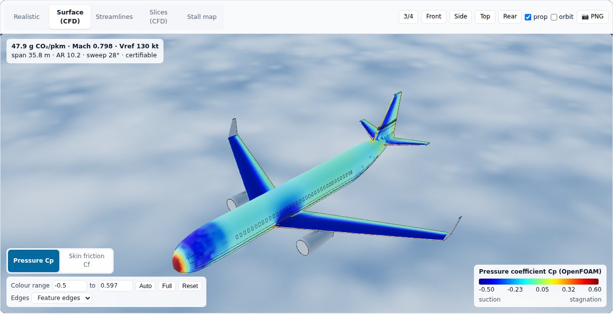
Controls under the modes: - Colour range: type the ends, or press Auto (1st to 99th percentile, the default) or Full (minimum to maximum). Each field, the lines and each slice group keep their own range. - Slice position: a slider through the slices of a stack, for example the wake planes of ExternalFlow. - Line density: shows an evenly spread share of the streamlines. - Edges: off, feature edges (creases above 30°) or wireframe.

studio-core.js holds the colour scale, colour bar, tubes, slice textures and edges. The apps load it from /studio/studio-core.js (the aircraft app's viewer is built on it), and its tick labels match the Python colour bar of the renders. Its tests run with node --test tests/js/studio_core.test.mjs.

How big a mesh? Measured with a closed surface carrying two fields, in headless Chromium with software WebGL on 4 CPU cores. That is a worst case: a laptop GPU draws frames much faster, while loading and recolouring run on the CPU anyway.

Triangles	scene.glb	Export	Page load	First frame	Field switch
25 k	0.7 MB	< 0.1 s	2.4 s	0.5 s	0.1 s
130 k	3.6 MB	0.1 s	1.9 s	0.8 s	0.3 s
260 k	7.3 MB	0.1 s	2.5 s	0.9 s	0.5 s
520 k	14.5 MB	0.2 s	2.3 s	1.4 s	0.8 s
1.04 M	29.1 MB	0.5 s	2.8 s	2.0 s	1.7 s

The file grows by about 28 bytes per triangle, plus about 2 bytes per triangle for each extra field. - Up to about 500 k triangles: stays interactive. - Above 1 M triangles (web_viewer(..., max_faces=1_000_000), the default): the page gets a decimated copy. The scene itself is not changed, and max_faces=None keeps every triangle. - For a smaller file: call scene.decimate(n) yourself. It uses vertex clustering and averages the fields, so thin features below the cluster size can close up.

Slices are stored as JSON grids, about 7 bytes per value. Keep them to a few hundred cells a side.

Fields, errors and deformed shapes in the apps: pp.viz.field_view

The apps show a result on its mesh with one shared page module, apps/_shared/static/shared/fieldview3d.js, served at /shared/fieldview3d.js and built on the same vendored three.js and studio-core.js. The library builds what it shows:

import pinneapple as pp
from pinneapple_analysis.validation.error_map import error_map, grow_region

em = error_map(mesh.points, pred, ref, regions={"clamp zone": grow_region(mesh.points, clamp, 0.2)})
fv = pp.viz.field_view(mesh, [
    {"name": "ref", "values": ref, "label": "FEM von Mises", "unit": "MPa", "group": "vm", "deform": "FEM"},
    {"name": "pred", "values": pred, "label": "ROM von Mises", "unit": "MPa", "group": "vm", "deform": "FEM"},
    {"name": "err", "values": em.error, "label": "|ROM − FEM|", "unit": "MPa", "kind": "error"}],
    deform={"FEM": u}, length_unit="m",
    markers=[{"name": "clamp", "kind": "bc", "points": mesh.points[clamp]}])
fv.glb(), fv.meta                  # the glTF (fields as vertex attributes) and its description
em.summary()                       # where the error concentrates, against the global number

• Colours. Values use the jet scale from their minimum to their maximum on the surface; fields of one group share a scale. Errors use the sequential error scale (ERR in studio-core.js, white = 0) from 0 to their 99th percentile, and the colour bar says when the maximum lies above it.
• Deformed shape. Each deform entry gives a nodal displacement. The page draws it with a scale factor. By default the largest displacement is drawn as 10 % of the body, and 1× shows the true scale. The undeformed shape stays as a grey wire.
• Markers. Boundary conditions, loads, error hotspots and other regions get coloured points and a label. A marker can belong to some fields only.
• Size. Above max_faces triangles (VIEW_MAX_FACES = 250 k by default) the surface is decimated, and the page says so. 250 k triangles is about 7 MB and a 0.5 s field switch in the table above.

Lighting presets, Sun shadows and planetary surfaces

studio.lighting holds lighting and sky presets that PyVista, Blender and the browser viewer share:

Preset	Sky	Sun	Used for
studio	grey-blue gradient	soft, 45°	the CFD renders (aircraft, Formula car)
lunar_south_pole	black	5°, 0.53° disc	the lunar south pole: within about 5.5° of the horizon at 86° S
lunar_low_sun	black	12°	long hard shadows, with small crater floors partly lit
lunar_day	black	30°	mid latitudes

How each renderer uses them: - PyVista: apply_pyvista(plotter, "lunar_south_pole", earth=True) adds the Sun, a weak regolith bounce light and, optionally, Earth at its 1.9° apparent size. - Blender: pp.viz.render(scene, "x.jpg", background="lunar_south_pole") lights the scene with one Sun lamp of the Sun's angular size and no sky light. - Browser viewer: scene.set_lighting("lunar_low_sun") makes the viewer draw the black sky and the low Sun.

studio.shadows bakes hard Sun shadows into heightfield terrains, independent of the renderer: - Self-shadowing: terrain_self_shadow marches towards the horizon along the Sun direction. - Cast shadows: cast_shadow projects vehicle and rock meshes along the Sun onto the terrain. - Shadowed points: points_in_terrain_shadow darkens meshes the terrain hides from the Sun.

Regolith is shaded with the Lunar-Lambert photometric function of McEwen (1991), which keeps it readable at grazing Sun angles where a Lambert surface turns black. studio.planetary.render_surface(SurfaceView(...)) puts it all together: terrain with baked photometry and shadows, a far-field ring, rocks, vehicle parts with their materials, optional field colour maps on the terrain and the parts with a colour bar, and Earth.

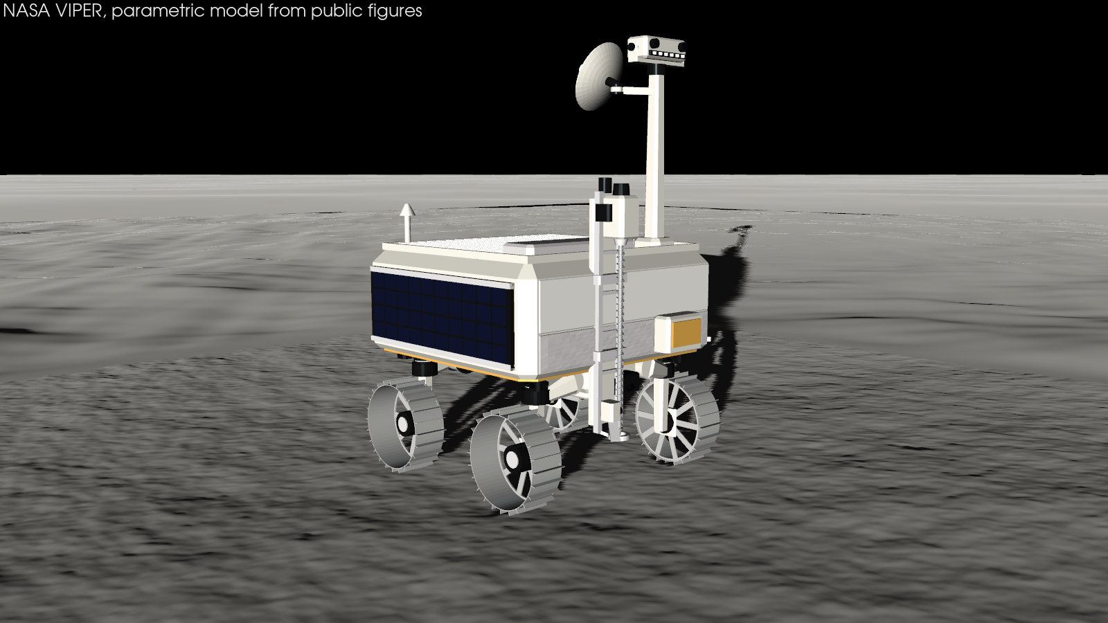
The lunar rover page (Lunar rover terramechanics in 3D) shows these in use.

Particle process videos

Thousands of spheres coloured by a value inside glass or steel equipment that moves (an impeller turning), rendered with Cycles point clouds, then composed with charts that draw themselves as time runs, a colour bar and a clock. Any Lagrangian result works: DEM, stirred tanks, fluidised beds, hoppers, sprays.

from pinneapple_simulation.numerical_solvers.particles import StirredTank, suspend
from pinneapple_tools.visualization.studio.particles import compose_video, render_particle_frames

tank = StirredTank(R=0.075, H=0.15)                                   # pitched-blade turbine, glass tank
res = suspend(tank, n=12000, d=3e-3, rho_p=1200.0, rpm=lambda t: min(400.0, 16.0 * t), t_end=30.0)
angle = ...                                                           # impeller angle per frame
pngs = render_particle_frames(res["frames"], 3e-3, "frames/", field_range=(0, 0.4),
                              equipment=lambda k: tank.surfaces(angle[k]))
compose_video(pngs, res["times"], "tank.gif", mp4=True, frame_dir="composed/",
              charts=[("Particles Top [%]", res["times"], 100 * res["top_fraction"]),
                      ("Stirrer Speed [RPM]", res["times"], res["rpm"])],
              colorbar=("Velocity Magnitude (m/s)", 0, 0.4))

frames is a list of dicts with x (n, 3) and a value per particle (speed or value). equipment(k) returns the surfaces of frame k as (name, vertices, faces, material) with material "glass", "liquid", "steel" or "grey". Surfaces keep their topology between frames, so only the vertices move. The MP4 goes through Blender's own encoder, so no ffmpeg binary is needed. The lab experiment particle_suspension runs the whole chain with checks: settling velocity against Schiller-Naumann, a divergence-free flow, particles kept in the tank, and the just-suspended speed against Zwietering.

Structural FEA with CalculiX: pp.fea

The same few lines for any part: a mesh, sets picked by geometry, one step, results as arrays, the post-processor figure or a Blender render.

import pinneapple as pp

m = pp.fea.FEModel.from_gmsh(pp.fea.geo_l_bracket(), size=0.0025)      # gmsh C3D10; or FEModel.from_box(...)
m.material = pp.fea.Material("steel", E=210e9, nu=0.3, density=7850.0)
base = m.nodes_where(lambda X: X[:, 2] < 1e-9)
top = m.nodes_where(lambda X: X[:, 2] > 0.08 - 1e-9)
res = pp.fea.solve(m, pp.fea.Static(fix=[(base, (1, 2, 3))], loads=[(top, (2000.0, 0, 0))]), "work/bracket")
res.u, res.stress, res.von_mises, res.reactions
modes = pp.fea.solve(m, pp.fea.Frequency(6, fix=[(base, (1, 2, 3))]), "work/modes")   # .frequencies, .modes

from pinneapple_simulation.numerical_solvers.solid_fem import fea_figure
fig, _ = fea_figure(res)                                                # deformed mesh, S Mises bands, legend

Steps: Static (point loads, face pressure, gravity, nonlinear geometry, plasticity through Material.plastic), Frequency, Buckle, Heat (fixed temperatures, film convection, surface flux). Faces come from m.faces_where(pred) on face centroids. ccx runs natively or in the bundled Docker image, and gmsh meshes any .geo script, OpenCASCADE booleans included. The lab experiment calculix_case checks five studies against closed-form references: a plate with a hole (Heywood), an L bracket (M c / I, mesh convergence), modes (Euler-Bernoulli), buckling (Euler) and a fin (1-D fin).

External flow: pp.cfd.ExternalFlow

flow = pp.cfd.ExternalFlow({"ahmed": pp.bodies.ahmed_body(25)}, speed=40.0, ground=0.0, half_model=True,
                           resolution="medium")
res = flow.solve("cases/ahmed", procs=4)      # write, snappyHexMesh, simpleFoam, read
res.coefficients                              # CD, CL, CS, pressure/friction split, per body, newtons
scene = res.to_scene()                        # skin Cp and Cf, streamlines by |U|/U∞, mid-plane and wake slices

Setup - Steady incompressible RANS: simpleFoam, k-ω SST, wall functions. - Bodies: a dict of (vertices, faces), an STL path or a Scene. - The domain and background cells scale with the bodies' length. resolution sets the surface refinement levels: coarse, medium or fine. - alpha and beta tilt the flow. - half_model adds a symmetry plane at y = 0. - wake_planes (default (0.25, 0.5, 1.0, 1.5) body lengths behind the bodies): the cross-flow slices, one stack per field in the viewer. - ground adds a road (True: at the lowest point of the bodies; a number: its height), moving with the flow unless ground_moving=False.

Results - Forces: pressure plus wall-function shear from the log law at the first cell. - Coefficients use ref_area; the default is the frontal area of the bounding box. - A FlowResult can be saved with res.save("result.npz").

Validation, Ahmed body, 25° slant, 40 m/s, half model, moving road

Mesh	Cells	CD	Time (2 cores)
coarse	0.15 M	0.321	4 min
medium	0.20 M	0.298	10 min
wind tunnel (Ahmed et al. 1984)		≈ 0.285

Needs OpenFOAM (v1912 and later tested). Set FOAM_BASHRC if its bashrc is not at /usr/share/openfoam/etc/bashrc. pp.cfd.openfoam_available() checks it. The aircraft case (pinneapple_design.aero.case3d) is built on the same pieces: write_flow_fields, snappy_dict, run_case and CaseFields, which provides wall forces, streamline tracing and plane sampling for any case.

Example: Formula car at 70 m/s

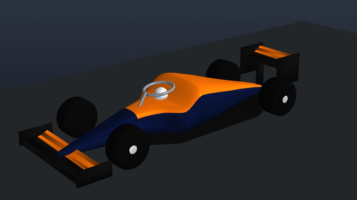
pinneapple_design.geometry.vehicles3d.FormulaCar is a parametric open-wheel car. It has:

• a tub and engine cover lofted from superellipse rings;
• a flat floor with a diffuser ramp;
• three-element front and rear wings built from NACA 4-digit sections, with a rear flap that opens for DRS;
• endplates, a helmet, a halo and four wheels.

cfd_bodies() groups the closed surfaces into body, floor, front wing, rear wing, helmet and wheels, so the forces come out per component. frontal_area() rasterises the front view, giving 1.68 m² for the default car.

examples/studio/06_formula_car_cfd.py [coarse|medium|fine] [procs] [drs] runs the half model through pp.cfd.ExternalFlow with a moving road at 70 m/s. It writes:

• the coefficients;
• the glTF scene and the browser viewer;
• PyVista stills;
• a Plotly page;
• a Rerun recording.

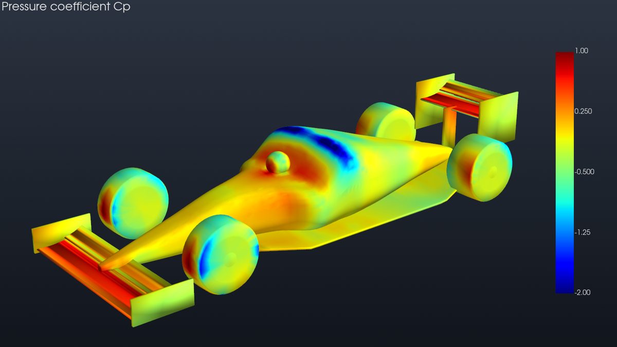
The pressure side of both wings is red. Suction peaks sit over the airbox, on the shoulders of the tyres and under the wing flaps.

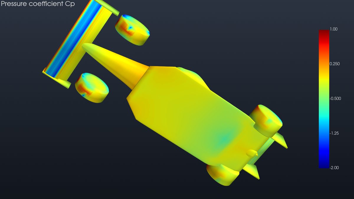
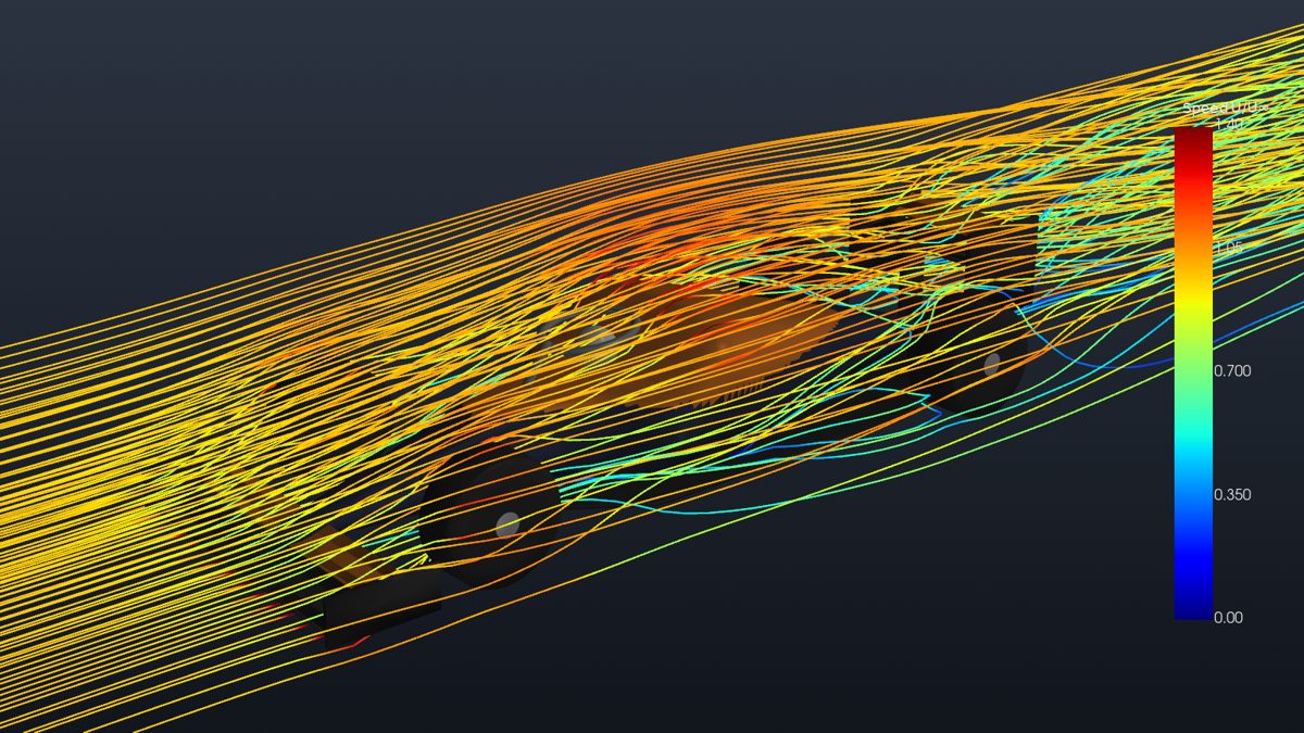
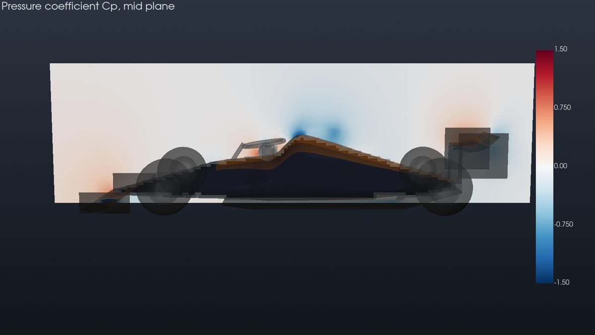
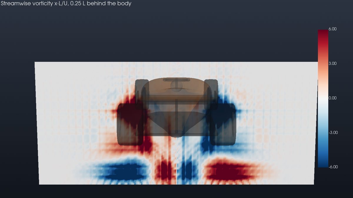
The wake plane 0.25 L behind the car shows two vortex pairs: one from the rear-wing tips and upper tyres, one low, from the rear tyres, the floor edges and the diffuser.

Medium mesh (0.21 M cells), 800 iterations, 4 cores, about 20 minutes per case:

Case	CD	CL	L/D	Drag at 70 m/s	Downforce at 70 m/s
DRS closed	0.596	-0.865	1.45	3.01 kN	4.36 kN
DRS open	0.580	-0.826	1.42	2.87 kN	4.09 kN

The coefficients use each case's frontal area (1.68 m² closed, 1.65 m² open), so compare the forces in newtons. Opening the flap cuts the rear-wing drag from 489 N to 214 N (−56 %) and its downforce from 1.80 to 1.41 kN (−21 %). The car's total drag falls by only 4.5 %, because the wheel drag rises by 144 N in the changed flow behind the wing.

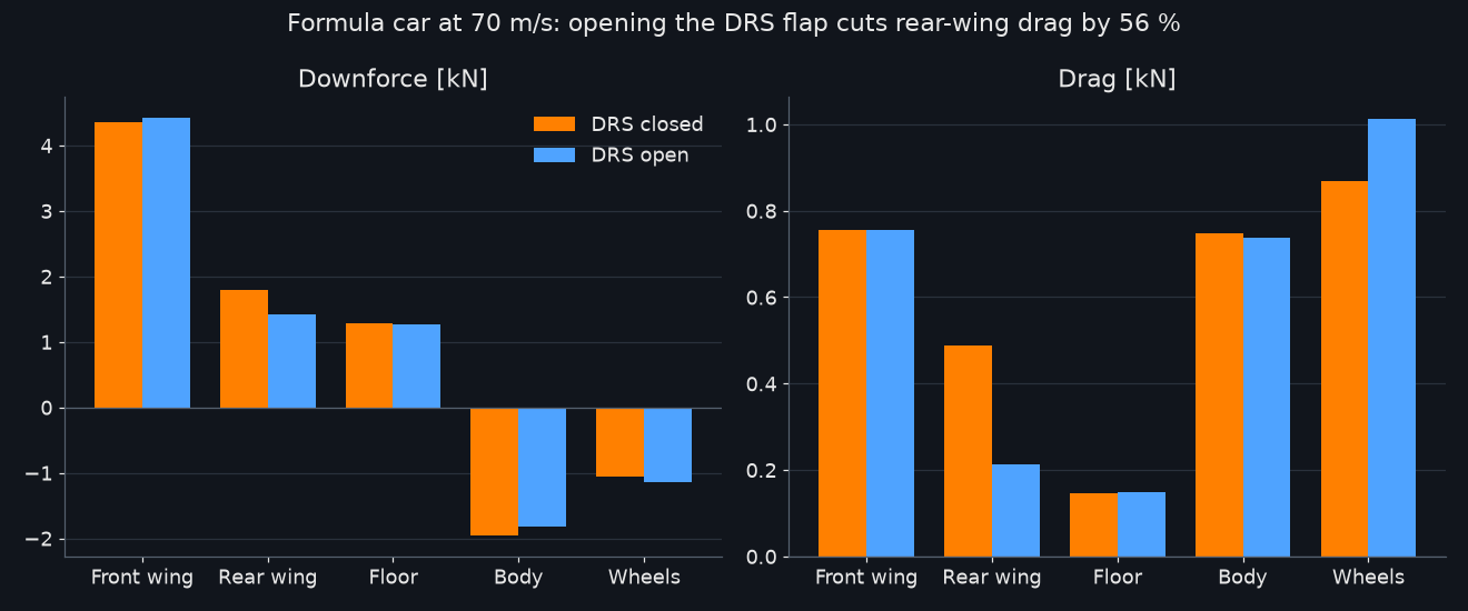
Per component, DRS closed (share of the net downforce):

Component	Downforce	Drag
front wing	4.35 kN (100 %)	0.76 kN
rear wing	1.80 kN (41 %)	0.49 kN
floor	1.28 kN (29 %)	0.15 kN
body	-1.96 kN (-45 %)	0.75 kN
wheels	-1.06 kN (-24 %)	0.87 kN
helmet	-0.04 kN (-1 %)	0.00 kN

The car is a simplified shape on a coarse mesh, so it shows the workflow; it is not a validated F1 aero model:

• The floor has no Venturi tunnels or edge vortex generators, so it gives under a third of the downforce, much less than on a modern car.
• The front wing carries almost all of the net downforce, while the tub and the wheels lift.
• Wall functions on 0.2 M cells resolve neither the wing boundary layers nor the tyre wakes.

Treat the numbers as a demonstration of the pipeline, not as a design result.

Bodies

pp.bodies.ahmed_body(slant_deg), sphere, cylinder and box return closed, outward-facing triangle meshes in metres, with x along the flow and z up.

Examples

• examples/studio/01_any_result_in_3d.py: a CalculiX result as glTF, USD, viewer and render.
• examples/studio/02_ahmed_body_cfd.py: from geometry to pictures, through OpenFOAM.
• examples/studio/03_airliner_with_cfd.py: the aero app's airliner with its OpenFOAM skin pressure.
• examples/studio/06_formula_car_cfd.py: the Formula car above, with DRS closed or open.