Adaptive ensembles of physics models

pinneapple_physics.ensemble.PhysicsEnsemble (also pp.ensemble.PhysicsEnsemble) selects and combines physics models case by case: neural operators (FNO, DeepONet), graph networks (MeshGraphNet), PINNs, numerical solvers and closed forms. It uses the same prequential core as the adaptive forecaster (pinneapple_physics.online_learning): Fixed-Share weights, AdaHedge over the learning and switching rates, adaptive conformal intervals. Every case is predicted with weights learned from earlier cases only, so the model choice cannot overfit.

from pinneapple_physics.ensemble import PhysicsEnsemble, from_callable, from_solution, from_torch

experts = [
    from_torch("fno", fno_model, to_input=lambda case: make_fno_input(case), from_output=lambda y, case: y[0]),
    from_torch("gnn", meshgraphnet, to_input=lambda case: make_graph(case), from_output=lambda y, case: y[0]),
    from_solution("pinn", pp.solve(problem, "pinn"), points=lambda case: case["points"]),
    from_callable("solver", lambda case: run_solver(case), cost=50.0),
]
ens = PhysicsEnsemble(experts, mode="select")      # or "combine"
for case in stream:
    out = ens.predict(case)                        # field, interval, per-expert fields, weights, active model
    ens.update(case, reference=high_fidelity(case))  # when a reference exists

What the weights can learn from

Signal	Argument	When to use
Reference field (sensor, experiment, high-fidelity run)	update(case, reference)	relative L2 error; validation campaigns, digital twins with sensors
Physics residual, no reference	residual_fn, residual_weight	operation without ground truth: models that violate the PDE lose weight
Cost	cost_weight, Expert(cost=...)	adaptive fidelity: the cheap surrogate while it is good enough, the solver when it is not
Physics residual of the current case, before predicting	residual_fn, residual_lookahead	regime changes: the choice reacts on the first new case instead of after past errors pile up

With mode="select" and predict(case, select_only_leader=True) only the leading model runs, except every explore_every cases, when all run so their errors stay current. Experts that raise or return non-finite values are left out of that case and scored with the worst loss.

router= adds physics-aware routing (pinneapple_physics.physics_audit.PhysicsAwareRouter): each expert's assumptions and training envelope are checked against the current case, the compatibility tilts the weights before predicting, and experts outside their physics sleep for that case without losing weight. See Physics audit.

prediction_checks={name: fn(prediction, case)} runs label-free checks on each model's prediction for the current case before choosing: a closure check of an LES, a cross-scale consistency check, a conservation check. Each returns a score in [0, 1] (or (score, reason)). A model whose score is below check_threshold is left out of that case but still scored, so its weight learns from the failure. The others are tilted by score ** check_strength. When every awake model fails, the router's escalate_from moves up a fidelity ladder. predict reports checks, failed_checks and escalated_by_checks.

Scales: which model can answer the question at all

A model trained or run at one resolution and filter represents the field at that scale and nothing finer. A small validation error does not make it fit for a question about smaller scales. pinneapple_physics.multiscale lets every expert declare its scales and every case declare the scales it needs:

• ScaleProfile: output filter (kind and width), grid spacing, closure, Reynolds range, time step and fidelity rung;
• ScaleQuery: the filter of the requested output, the Reynolds number and the time scale;
• ScaleAwareRouter: a model asked for scales below the ones it resolves sleeps. A filter it cannot reproduce by post-filtering its own output is tilted down. The lowest fidelity rung that covers the case is used (surrogate, then LES with a closure, then a resolved solver), and the router moves up a rung when the closure checks fail.

The filters, the closure tests, the multiscale residuals and the experiment on 2-D turbulence are described in Multiscale ensembles: scales, filters and closures.

Other options: conserve=(weights, target_fn) projects the combined field onto a conserved total; min_weight keeps near-zero weights out of the "combine" average; point_weights gives quadrature weights for the norms. fit_static_weights(predictions, references) fits fixed convex weights on a validation set and reports their cross-validated error next to each single model.

Results (advection-diffusion with exact solutions, pinneapple_physics.advection_diffusion_1d)

150 cases whose diffusivity moves through three regimes; every learned model was trained on one regime only (examples/physics_ensemble/fno_pinn_gnn_solvers.py):

	low nu	mid nu	high nu	all cases
FNO (trained on low nu)	0.57 %	4.4 %	40 %
MeshGraphNet (trained on mid nu)	19 %	16 %	38 %
PINN (high nu, physics loss only, no data)	16 %	13 %	6.5 %
upwind FD	4.1 %	3.4 %	2.5 %
Lax-Wendroff FD, coarse grid	2.5 %	1.2 %	0.10 %	1.25 % (best single model)
Adaptive ensemble, select	0.57 %	2.0 %	0.10 %	0.88 %

Relative L2 error of the space-time field. 90 % intervals covered 93 % of the points. In the tests (tests/test_physics_ensemble.py) the residual-only mode (no reference at all) removes the out-of-distribution FNO in the high-diffusion regime, and the cost-aware lazy mode cuts the compute by more than 70 % against running every model while keeping the error low. With CPU-sized training the MeshGraphNet stays the weakest expert; the ensemble learns to ignore it. In "combine" mode a model that fails badly still costs a little during a regime change, so "select" is the better default when some experts can be far off.

The PDE residual is a good detector of failure (it flags the out-of-distribution FNO at once), not a ranking of the most accurate model: a learned field can have a larger residual than a slightly less accurate numerical solution.

Five model families and an animated view

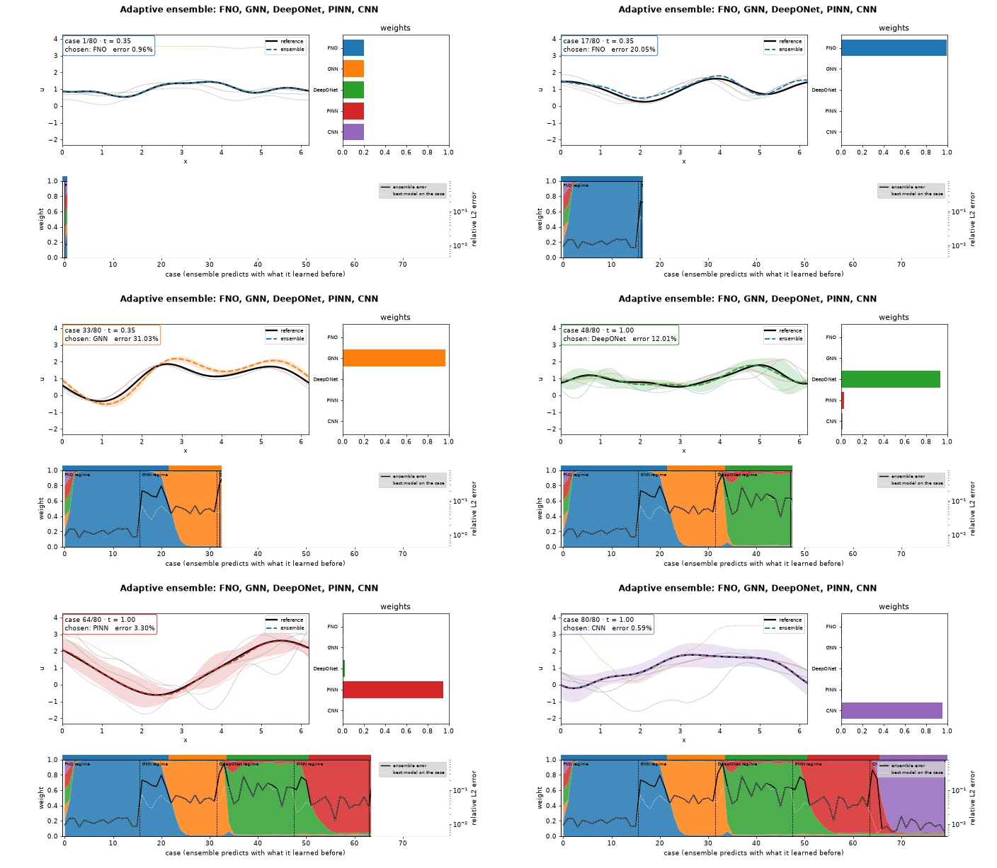
examples/physics_ensemble/five_model_families_gif.py puts an FNO, a MeshGraphNet (multiscale ring graph), a DeepONet, a PINN (physics loss only) and a dilated 1-D CNN in one ensemble. Each is trained on its own regime of advection speed and diffusivity; the stream of 80 cases drifts through the five regimes. Relative L2 error per regime (select mode, 16 cases each):

regime (training data of)	FNO	GNN	DeepONet	PINN	CNN	ensemble
FNO (c = 1, low nu)	1.2 %	240 %	38 %	45 %	72 %	1.2 %
GNN (c = 0.5, high nu)	18 %	5.4 %	18 %	26 %	74 %	10 %
DeepONet (c = 0, mid nu)	37 %	63 %	11 %	18 %	29 %	16 %
PINN (c = -0.5, high nu)	39 %	28 %	16 %	4.2 %	51 %	7.0 %
CNN (c = -1, low nu)	128 %	153 %	37 %	27 %	0.96 %	4.7 %
all cases				24 % (best single)		7.8 %

The ensemble switches to the right family 2 to 6 cases after each regime change (the gap to the diagonal is that delay); no single model comes close over the whole stream. 90 % intervals covered 90 % of the points.

Detecting the regime change before the errors pile up

The weights above learn only from cases already seen, so every switch lags. residual_lookahead adds a signal that exists at prediction time: before choosing, each model's PDE residual on the current case is compared with a reference level for that model, and the weights are tilted by (r / reference) ** -residual_lookahead. A model whose residual is far above its reference has left its domain; the learned weights still decide between models whose residuals look normal. The reference is, in order of preference:

• residual_baseline: the level each model has in its own domain, measured before operation on a few of its training or validation cases (residual_baseline(experts, {name: domain_cases}, residual_fn));
• otherwise the model's median over the last lookahead_window cases.

Same five models and stream, five seeds:

choice of model	mean error	cases with the wrong model (of 80)	cases taken by a model outside its regime	cases until the right model, per regime change
oracle (best model of each case, in hindsight)	0.045	0	0	0
past errors only (the GIF)	0.081	13-19	12-15	4-6, 2-3, 3-4, 2-3
+ residual against each model's recent history, residual_lookahead=3	0.051	4-9	2-6	1-2, 0-1, 0-1, 0
+ residual against its training-regime level, residual_lookahead=10, residual_baseline	0.049	3-5	0-3	0, 0-2, 0, 0

The recent history is out of domain right after a regime change, so it cannot tell apart two models whose residuals drop together: the GNN and the PINN were both trained at high diffusivity, and on the first case of the GNN regime the history version hands it to the PINN. The in-domain level separates them. Comparing raw residual levels across models (lookahead_reference="experts") also switches at once, but it ranks models by how well they satisfy the PDE, which is not how accurate they are: a numerical scheme that solves its own discrete equation has a tiny residual and a larger discretisation error than a well-trained neural operator (in the test suite it takes the FNO's own regime away from it).

examples/physics_ensemble/five_model_families_gif.py takes main(lookahead=10.0) to run the calibrated version, and examples/physics_ensemble/compare_lookahead_gif.py runs the three on the same cases and writes the figures below (one run; every run retrains the models, so the numbers move a little).

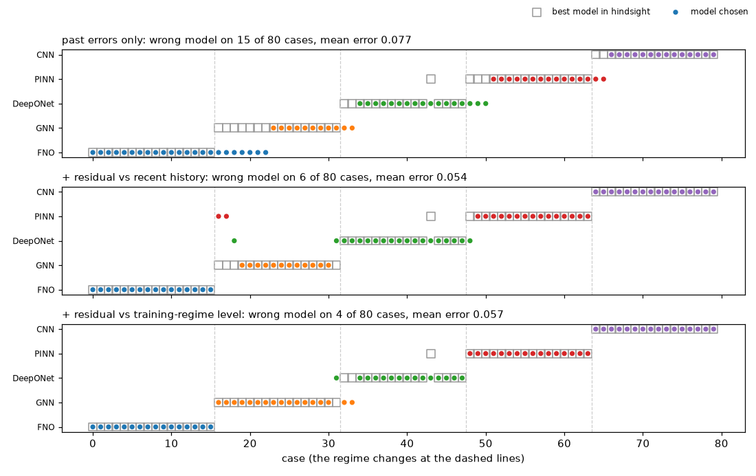
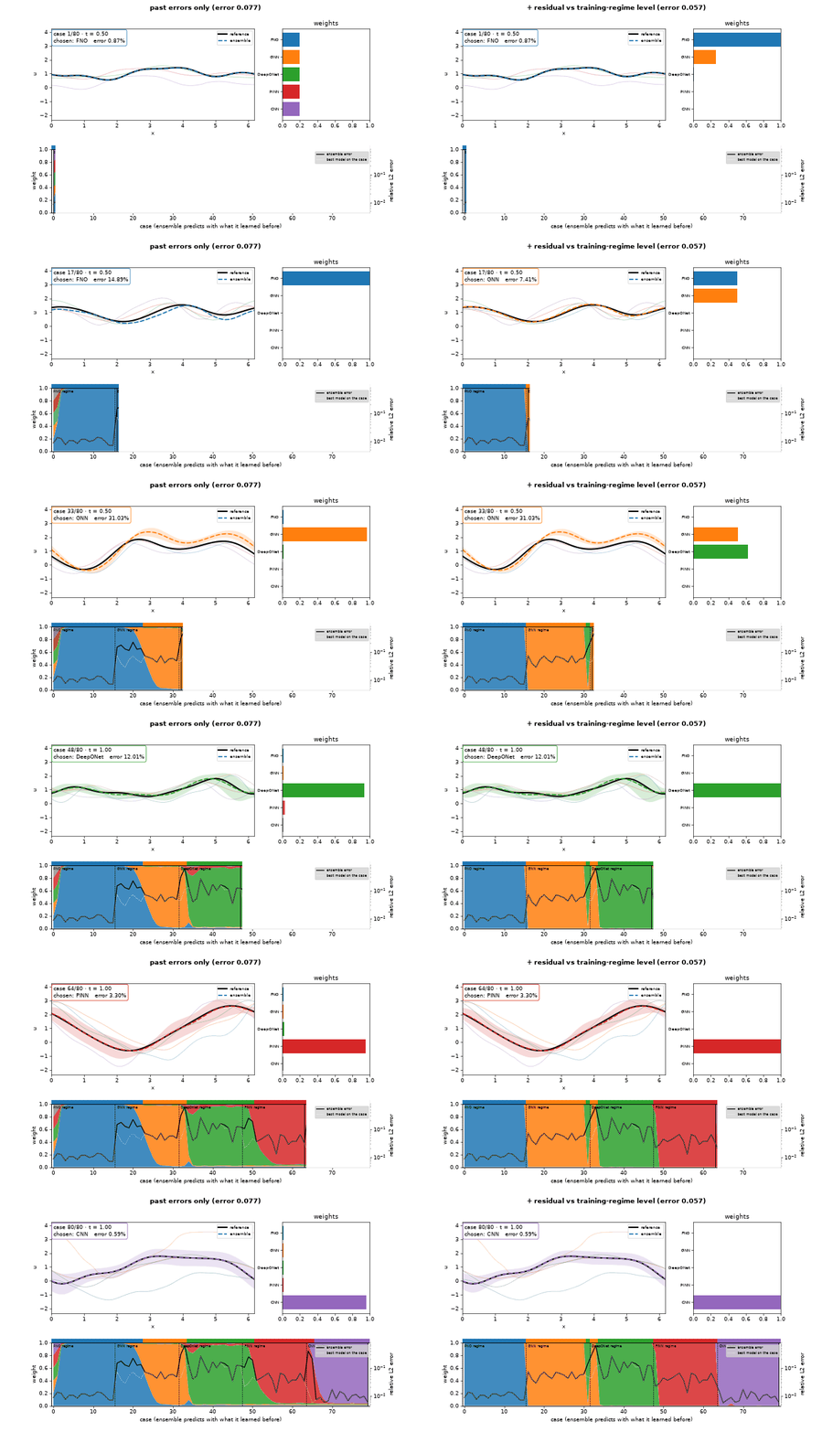
What is still wrong: the GNN-to-DeepONet change is the weak one (in this run the choice moves one case early and then lags two cases), because the GNN's residual on low-diffusion cases does not rise clearly above its own level. And a model can be wrong in a way the PDE residual does not see (a wrong boundary condition, a wrong parameter that is consistent with the equation); then only the reference errors catch it.

Regime change or sensor noise?

A noisy reading raises the residual too, and the residual of each model by a different amount, so the current-case residual alone also switches the model on noise. Two options keep the early switch at real regime changes and drop the false ones:

• measurement_check(query) -> bool: physics on the reading, before any model is involved. True means the measurement itself is implausible (a failed mass or energy balance across redundant sensors, an impossible jump, energy where a physical state has none). A flagged reading is predicted with the learned weights only and teaches nothing: no weight update, no interval calibration, no residual history. EnsembleRun.suspect lists them.
• lookahead_persistence=N: the residual of a model counts only when its last N readings agree (all above or all below its reference). A real regime change persists; a noise spike does not. The cost is N - 1 readings of delay.

Five-family stream with 15 % noisy readings (the measured input and the measured response), one run of examples/physics_ensemble/sensor_noise_gif.py, errors measured against the true field:

choice of model	wrong model on noisy readings	flagged readings	mean error
current-case residual only	8 of 12	0	0.083
+ physics check of the reading (measurement_check)	0 of 12	12 (all noisy, no false alarm)	0.067

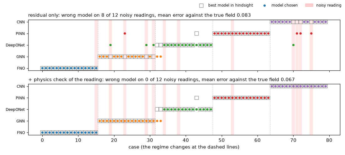
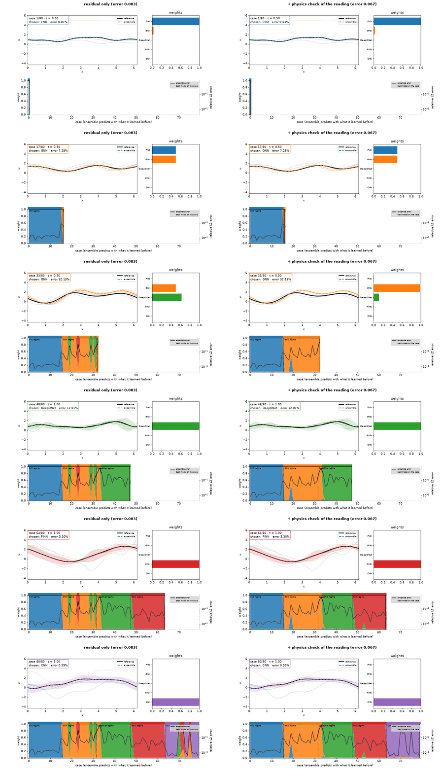
Over five seeds the same comparison gave 6.2 and 2.0 wrong models on 12 noisy readings (0.079 and 0.059 mean error); lookahead_persistence=2 alone gave 1.4 and 0.072. The check here is easy, because white noise on a smooth state is easy to see; in a plant the equivalent is a balance across redundant sensors, and slow sensor drift, which looks like a real process drift, is the hard case that only real process data can settle.

pinneapple_physics.ensemble_viz.animate_ensemble(run, references, "ensemble.gif") animates any run made with run(..., keep_predictions=True): the reference field against the ensemble's prediction (coloured by the chosen model, with its interval and every expert as a faint line), the weights sliding between cases, and a timeline of weights, chosen model and error revealed case by case. Space-time fields (n_t, n_x) are stepped through time so the waves move; 1-D fields are shown one frame per case.